Manage Your Site Inventory For Free with Google Drive (Part III)

Part 3 of our multi-part series on how to create a FREE inventory system using Google Drive will dive deep into data manipulation.  As a refresher, Part one talked about the overall process summary and part 2 discussed setting up a Google Form to easily grab data from anyone or anywhere that has an internet or mobile connection.

View Your Form Data

After setting up your Google Form to your liking, you’ll notice that a Google Sheet is automatically created to store the data that’s input and submitted into your Form.  A Google Sheet is a spreadsheet program that is extremely similar to Microsoft Excel, which I’m sure you all have used at some point in your life.  This data is a great log of entry, but we’ll have to take it a few steps further to create our system.

Reference Form Data in Another Sheet

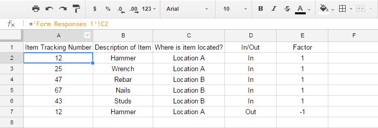
So, to make your form data into a live, automatically updating inventory system, first go to the tab titled “Sheet 2”, and reference your data from the “form responses” tab using an equation like the one in the picture below.  It’s important to have your “inventory #” be in the first column for future steps, which is why I rearranged the order.

Assign a Factor

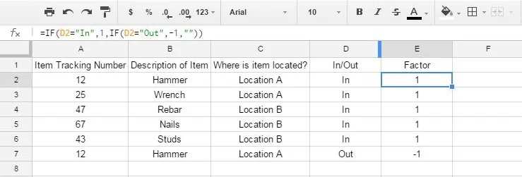
Next, after you reference all of your form data like above, create a new column titled “factor”.  We need to assign a factor for an item that is entering our inventory and one that is leaving.  The IF-statement formula shown below tells the spreadsheet to assign any item that says “in” a factor of 1 and any item that says “out” a factor of -1

Create a Pivot Table

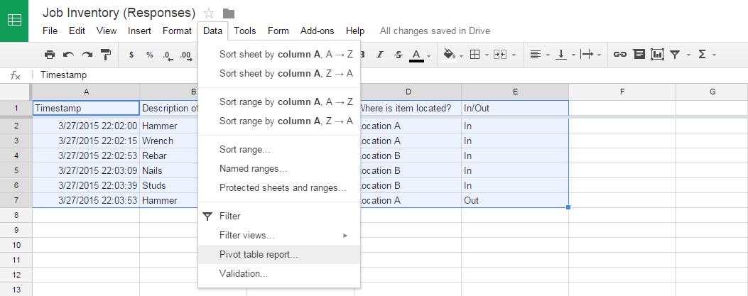
Select all of your data in sheet 2 plus a few hundred more rows for future additions, and create a pivot table, which will be embedded on a separate sheet.  A pivot table compiles data from another table and easily compiles it for easy to read summaries.  We will use this to sum our quantities (you’ll notice item #12 has a line that says “in” and also a line that says “out”).

Input the settings as shown below into your pivot table.  Item 12 now shows a quantity of zero, indicating that that specific item came into our inventory and then left.

Create Final Inventory Spreadsheet

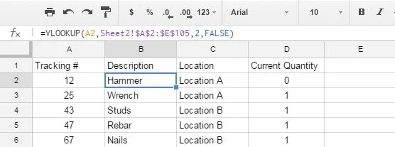
Finally, create one final sheet, this will bring everything together.  First, reference the item numbers in the pivot table sheet like we did for sheet 2, to transfer those numbers to this new sheet.  Next, we’re going to use one of my favorite spreadsheet formulas, VLOOKUP, which will allow us to grab data that corresponds to the item number from other sheets without entering it manually.  Below, I show you how I set up my VLOOKUP function for the Item Description.  The basic idea of this formula is so: =VLOOKUP(cell you wish to lookup (in our case: item number), the range of data that you wish to look through, the column you want to reference (count columns starting with the first one), whether you want an exact match or a similar match (we want exact, so enter FALSE)).  When you type in =VLOOKUP into your form, Google also shows you a helpful popup screen which explains further.  DO that for all columns, but remember to reference the pivot table you created when you get to the “Current Quantity” column.

And there you have it; by using some basic formulas, you have created a live updating inventory system for free.  Once you’re comfortable with setting up this very basic inventory, feel free to explore the many other options Google Forms and Google Sheets have available and make this form your own.

Still have questions or need some help getting yours to work? Comment below!